
Visualize your data, analyze your results, map your statistics, and find the data you need! Come visit us in Perkins 226 (second floor Perkins) for a consultation or contact us online (email: askdata@duke.edu or twitter: duke_data OR duke_vis). We look forward to working with you on your next data driven project.
New Data Lab Opens- August 2012
http://library.duke.edu/data/about/lab.html
With 12 workstations with dual 24″ monitors and 16 gigs of memory, the new Data and GIS lab is ready to take on the most challenging statistical, mapping, and visualization research projects. The new lab also features a flatbed scanner for projects moving from print to digital data. Lab hours are the same hours as Perkins Library (almost 24/7).
Visualize This! New Data Visualization Program
Perkins Library is proud to introduce Angela Zoss our new Data Visualization Coordinator. Schedule a consultation, attend a workshop, or learn more about research in Data Visualization at Viz Forum this fall.
New workshops for Fall 2012
http://library.duke.edu/data/news/index.html
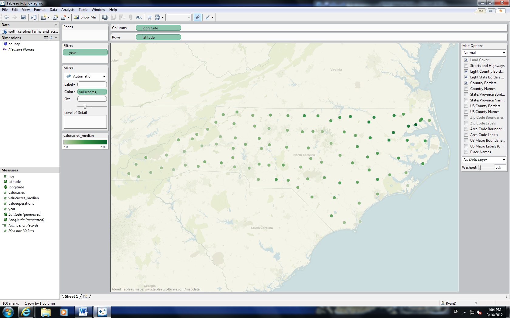
Learn about data management planning. Apply text mining strategies to understand your documents. Visualize your data with Tableau Public, or map your results using ArcGIS or Google Earth Pro. A new series of workshops connects traditional statistical, geospatial, and visualization tools with web based options. Register online for our courses or schedule a session for your course by emailing askdata@duke.edu
- Data Management Planning (Data Management/Grants)
- Excel Charts (Data Visualization in Excel) (Data Visualization)
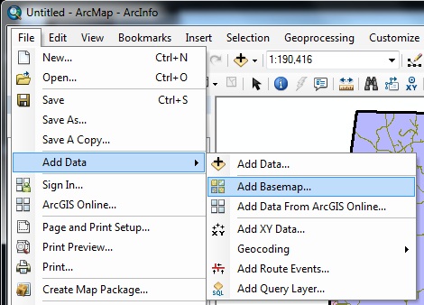
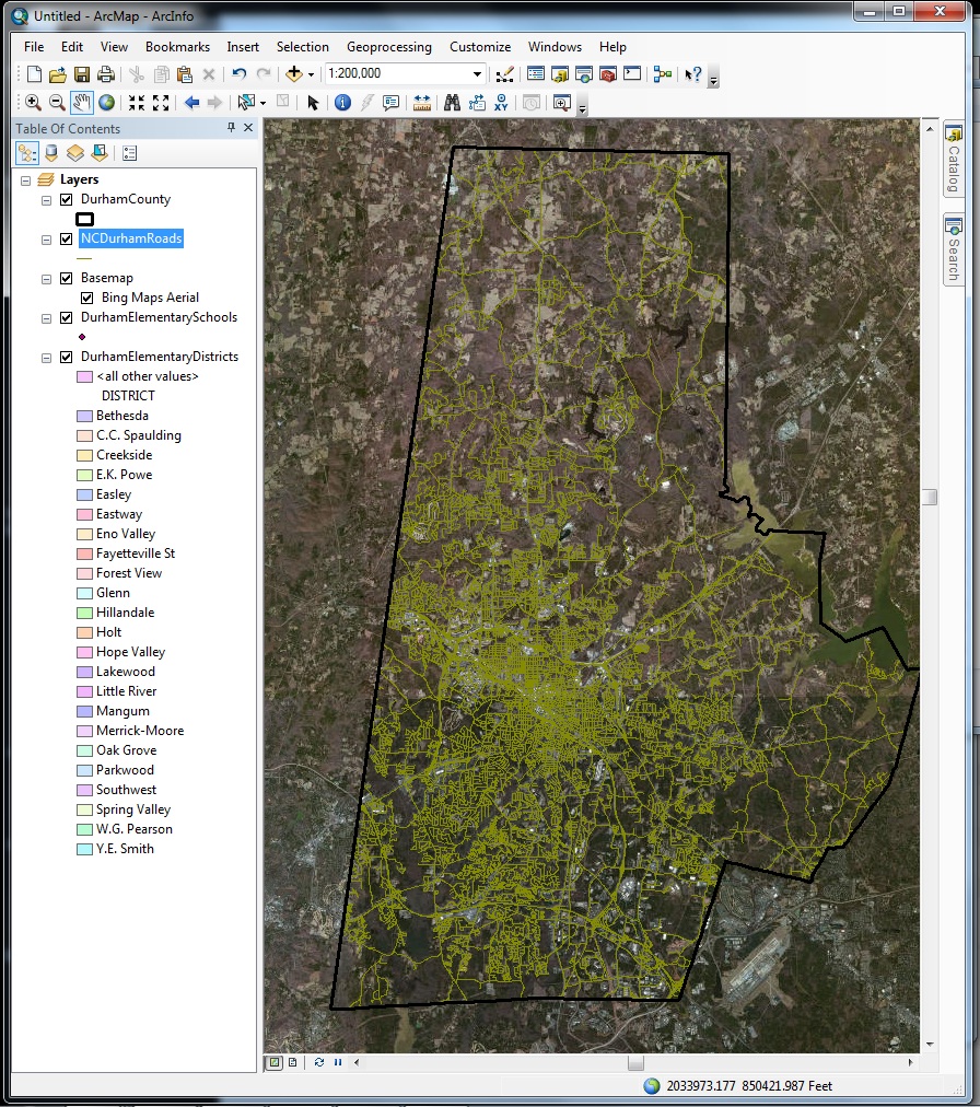
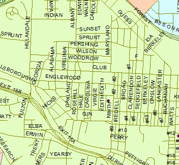
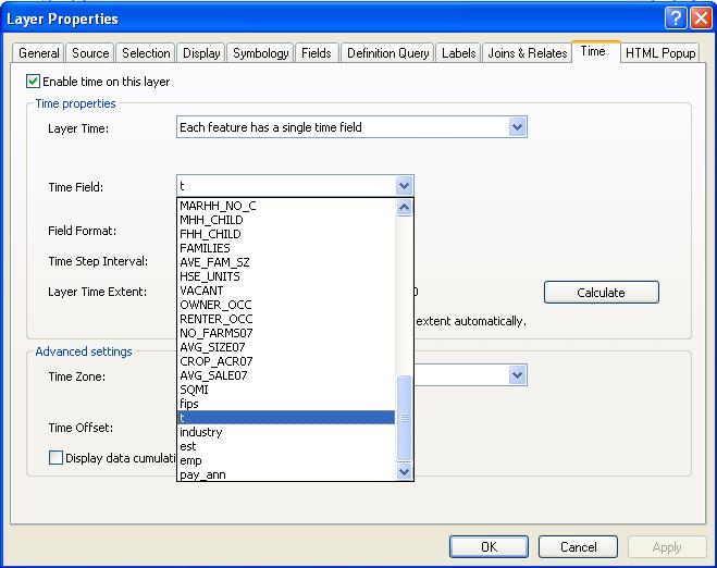
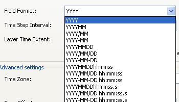
- Introduction to ArcGIS (GIS /Data Visualization)
- Intro to Data Visualization (Data Visualization)
- Intro to Text Analysis (Text Mining/Datavis)
- Historical GIS (Spatial Humanities/ GIS)
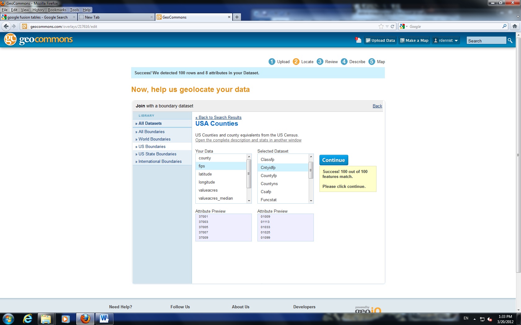
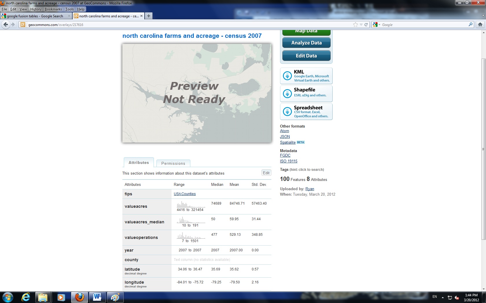
- Online Mapping (Fusion Tables, Google Earth, Geocommons) (Geographic Information Systems / Data Visualization)
- Stata Review (Statistics/Data Management)
- Tableau Public (Data Visualization)
Bloomberg Professional News and Financial Data
http://blogs.library.duke.edu/data/2011/08/29/bloomberg-has-arrived/
If you missed last fall’s Bloomberg service – Duke Libraries in pleased to announce the installation of three Bloomberg financial terminals in the Data and GIS Lab in 226 Perkins. The terminals provide the latest news and financial data and include an application that makes it easy to export data to Excel. Access is restricted to all current Duke affiliates. Training on Bloomberg is currently being planned for the last week of September. Please email askdata@duke.edu to reserve a space at the training session.
Get help with Data Management Planning
http://library.duke.edu/data/guides/data-management/index.html
Data and GIS has launched a new guide that provides guidance for researchers looking for advice on data management plans now required by several granting agencies. The guide provides examples of sample plans, key concepts involved in writing a plan, and contact information for groups on campus providing data management advice. In addition, we offer individual consultations with researchers on data management planning.
New Collections for Fall 2012
http://library.duke.edu/data/collections/new.html
Contact Us! – askdata@duke.edu


 Data visualization and data management represented the core themes of the
