Category Archives: census

Standardizing the U.S. Census

Census Tract Boundary Changes
(https://datasparkri.org/maps/)

The questions asked in the U.S. Census have changed over time to reflect both the data collecting needs of federal agencies and evolving societal norms. Census geographies have also evolved in this time period to reflect population change and shifting administrative boundaries in the United States.


Attempts to Provide Standardized Data

For the researcher who needs to compare demographic and socioeconomic data over time, this variability in data and geography can be problematic. Various data providers have attempted to harmonize questions and to generate standard geographies using algorithms that allow for comparisons over time. Some of the projects mentioned in this post have used sophisticated weighting techniques to make more accurate estimates. See, for instance, some of the NHGIS documentation on standardizing data from 1990 and from 2000 to 2010 geography.

NHGIS

The NHGIS Time Series Tables link census summary statistics across time and may require two types of integration: attribute integration, ensuring that the measured characteristics in a time series are comparable across time, and geographic integration, ensuring that the areas summarized by time series are comparable across time.

For attribute integration, NHGIS often uses “nominally integrated tables,” where the aggregated data is presented as it was compiled. For instance, comparing “Durham County” data from 1960 and 2000 based on the common name of the county.

For geographically standardized tables,  when data from one year is aggregated to geographic areas from another year, NHGIS provides documentation with details on the weighting algorithms they use:

1990 to 2010 Tract changes in Cincinnati
(https://www.nhgis.org/documentation/time-series/1990-blocks-to-2010-geog)

NHGIS has resolved discrepancies in the electronic boundary files, as they illustrate here (an area of Cincinnati).

Social Explorer

The Social Explorer Comparability Data is similar to the NHGIS Time Series Tables, but with more of a drill-down consumer interface. (Go to Tables and scroll down to the Comparability Data.) Only 2000 to 2010 data are available at the state, county, and census tract level.  It provides data reallocated from the 2000 U.S. decennial census to the 2010 geographies, so you can get the earlier data in 2010 geographies for better comparison with 2010 data.

LTDB

The Longitudinal Tract Database (LTDB) developed at Brown University provides normalized boundaries at the census tract level for 1970-2010.  Question coverage over time varies. The documentation for the project are available online:

NC State has translated this data into ArcGIS geodatabase format.  They provide a README file, a codebook, and the geodatabase available for download.

Do-It-Yourself

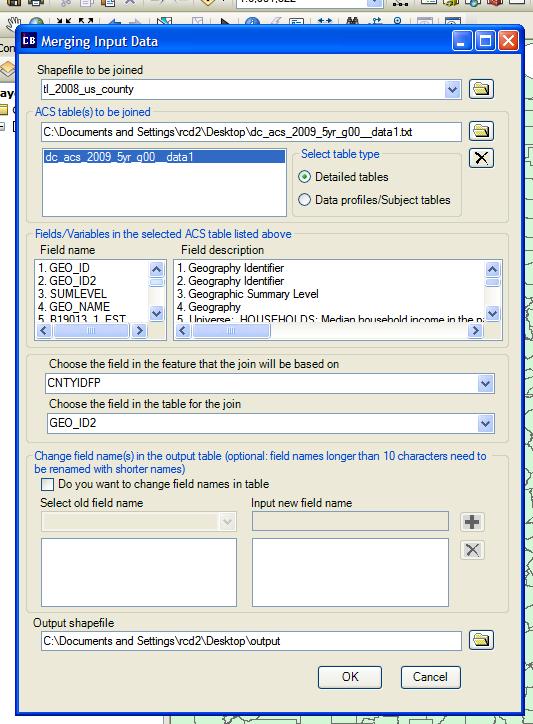
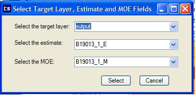
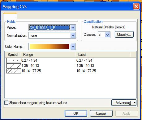
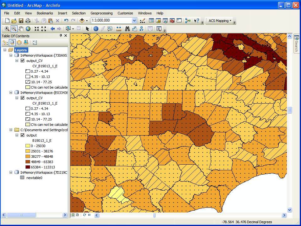
If you need to normalize data that isn’t yet available this way, GIS software may be able to help. Using intersection and re-combining techniques, this software may be able to generate estimates of older data in more recent geographies.  In ArcGIS, this involves setting the ratio policy when creating a feature layer, to allow apportioning numeric values in attributes among the various overlapping geographies. This involves an assumption of an even geographic distribution of the variable across the entire area (which is not as sophisticated as some of the algorithms used by groups such as NHGIS).

Another research strategy employs crosswalks to harmonize census data over time. Crosswalks are tables that let you proportionally assign data from one year to another or to re-aggregate from one type of geography to another.  Some of these are provided by the NHGIS geographic crosswalk files, the Census Bureau’s geographic relationship files, and the Geocorr utility from the Missouri Census Data Center.

You can contact CDVS at askdata@duke.edu to inquire about the options for your project.


Welcome to the Current Population Statistics on the Web

Duke University recently acquired access to the online version of its Current Population Statistics (CPS) CD-ROM collection to facilitate easy access to CPS data (Unicon’s CPS Utilities on the Web).  This blog post will walk through the basic data extraction process.  The interface is comparable to that provided by the CD, and users of this collection will find the interface and powerful.  Please note that the instructions provided on the web site are very important to read, particularly for those unfamiliar with the CPS CD version.

Create an Account

When you visit the Unicon site (http://unicon.com/), click the “CPS on Web” link to the left, then click the Register button.  You will have to enter some information to complete the registration process.

Once complete, submit the information.  Once the registration window closes, choose the CPS series (or month) you wish to query, and log in to the system.


1Navigation and Data Extraction

Once logged in, you will see a popup window like that shown in the image to the right.  For a typical data extraction, the following steps are advised.

1) First, click the Set Option button and chang4e the timeout to at least 300 seconds.  This will ensure successful data extraction.

2) Next, click the Make an Extraction button, followed by the Request Editor button on the next page.  You should see a page similar to that below (all variables used in your prior extraction will be listed).

23) Remove any variables you do not need.  Next, make certain the variable you wish to include is selected at the top and click “Add Variable(s).”  Alternatively, if you already know the names of the variables, you may type them into the boxes provided on the page.

4) Once all variables are added to the selection, click Continue.  On the following page, specify the output format for the dataset.  Once complete, be certain to select one or more years (at the top).  After you have selected years, click the Extract button.

5) On the following page, you will be presented with a list of variables by year.  As variables change across years in some cases, not all selected variables may be present for each year.  When selecting variables, checking the “View Documentation” checkbox at the top will allow for browsing of available years.


Other Useful Tools

– The Make a Table button allows for the construction of crosstabs of observations, means, and other statistics.  This is helpful if the goal is to locate variables for analysis or if there is a choice between two or more variables.

– The Make a Graph button is also useful for data exploration.  The program provides the ability to construct hsitograms, line charts, scatter ploys, pie charts, and bar charts.  Basic summaries of a variable can also be generated from this page.

– If your data need to be weighted to represent the US population, be certain to select the appropriate weight under the Apply Weights button before extraction.

– Subsets of individuals can also be produced under the Specify Universe button.  For example, a specific race or gender can be specified to reduce the sample to what you need.

ACS Mapping Extension for ArcGIS

The Census Bureau’s American Community Survey provides a continuous measure of the community demographics in the US.   A  new extension provided by the Department of Geography and Geoinformation Science at Geroge Mason University enhances the mapping of ACS by data by allowing researchers to visualize both survey estimates while revealing the level of uncertainty in the estimates.  ACS Mapping Extensions is an ArcGIS addon available for both ArcGIS 9.3 and 10.  This post provides a brief overview of installation, setup, and use.  Detailed technical assistance is provided by the extension.


Installation
1) Once you download the program, you will want to install and note the installation directory.  In ArcGIS, select Customize from the menu bar, and click Customize Mode….  Then select “Add from file…” and navigate to the installation directory.  Once in this directory, select the “ACSMapping.tlb” file.


2) Before you leave the Customize window, be sure to check the “ACS Mapping Tools” toolbar.  You will have a new “ACS Mapping” toolbar added to your window.


Setup
1) The “Documentation” option in the “ACS Mapping” toolbar provides detailed instructions for downloading ACS data and boundary files.  Follow these instructions to the letter and to their entirety.  With respect to boundary files, the TIGER 2008 county boundaries were used for this example.


2) Add the boundary layer to a blank map and select “Join ACS Table(s) with Shapefiles” option in the “ACS Mapping” toolbar.  In this example, I have downloaded county boundaries and county-level median income data from the 2005-09 ACS.  In this figure, the first two fields indicate the items to be joined, one table to one shapefile.   “CNTYIDFP” represents the FIPS code in the boundary file, and “GEO_ID2” is the corresponding code in the ACS table.  Once you’ve set an output location, select “OK.”


3) Finally, you will want to apply a symbology to the layer.  In this case, I chose the median income estimate and 5 total categories.  The following figure shows what my map looks like at this point.


Mapping ACS Estimates with Coefficients of Variation

1) The tools are located under the “Mapping Data Uncertainty” option in the ACS Mapping toolbar.  The first option, “Overlay CVs with Estimates,” will allow you to visualize the uncertainty of estimates at the same time as the estimates themselves.    As noted by the documetation provided by the ACS Mapping Extension web site, ACS provides a margin of error that produces a confidence level of 90%.  This tool will convert these data into coefficients of variation that will allow you to assess the quality of the estimates.


2) Select the target layer to whcih you added symbology, select the variable that stores the estimate to be calculated, and finally, select the variable that stores the margin of error (suffix = “_M”).


3) After you click the “Select” button, you will be presented with the new Symbology options for the new coefficients of variation layer to be generated.  In this case, I retained the automatic selections and hit “OK.”


4) Zooming in to central North Carolina, one can see not only that the Research Triangle Area has relatively high incomes compared with much of North Carolina, but that coefficients of variation are lower than thay are for parts of northern North Carolina and southern Virginia.


Measuring Singificant Differences in Income
1) The second option, “Identify Areas of Significant Differences,” allows you to assess whether there is a significant difference between one spatial unit and all other spatial units for a given variable.  In order for this option to work, you must select one specific spatial unit.  In this example, I selected Durham County and will assess whether there are significant differences in median household income in the region.


2) First, select the target layer for which you selected a single feature.  You want to verify the estimates and margin of error variables, and you can adjust the confidence level from the default 90%.  Select OK.


3) The output is represented by four different symbologies.  First, your chosen county is filled with dots.  All counties that are significantly different are striped, while all those that are not are empty.  Finally, when significance cannot be determined, the original color fill is replaced with a new color.  In this case, median household income is not significantly different between Durham and Chatham counties.  However, this could be due to small differences or large margins of error in one or both counties.