Time series data is easy to display as a line chart, but drawing an interesting story out of the data may be difficult without additional description or clever labeling. One option, however, is to add regions to your time series charts to indicate historical periods or visualization binary data.
Here is an example where a chart of annual U.S. national economic indicators has been enhanced with regions that also indicate contractions in the U.S. business cycle – roughly speaking, economic recessions.
To create this chart, all of the indicators were averaged by year and, where necessary, adjusted for inflation using a conversion factor. Download the time series data Excel file for the data and the chart to follow along.
First, to set up the basic line chart, hold Ctrl (PC) or Cmd (Mac) while you select the following columns:
- D (stock price index over CF…)
- E (avg. annual unemployment…)
- G (GDP over CF…)
- I (debt over CF…)
- K (interest rate * 10)
- L (years economy is in decline)
Youll notice that the columns are color coded. Some colors apply to multiple columns; this is because the values that appear on the chart have been calculated by transforming the raw data in some way. Each line on the final chart thus corresponds to one or more columns of data used to produce the values. Transforming the values helps us by normalizing the values (i.e., adjusting for inflation) or scaling the data series itself (making it possible to see the relationships between many different indicators on a single graph, despite wide variations in the ranges of values).
When we select the six columns above and insert a line chart, we get a rather ugly line chart.
We’ll make several changes to improve this:
- Change the “years… in decline” series to an area chart
- Select and adjust the x axis labels and ticks
- Adjust the y axis range
- Customize the color, label, and order of the data series
The basic mechanism of the colored regions on the chart is to use Excel’s “area chart” to create rectangular areas. The area chart essentially takes a line chart and fills the area under the line with a color. If we have a continuous horizontal line as a data series, we will create a large colored rectangle on the chart. To have breaks in the rectangle, we simply need to leave some of the years blank (without values in the cells). To select the appropriate values for column L, we first found the maximum value for the other data series and determined that a value of 20 would create bars starting above the other data series.
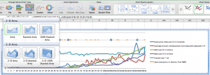
To produce the colored regions that indicate contractions in the business cycle, we take the series that was created from column L and turn it into an area chart.
- Right-click on any data point in the series or on the legend entry
- Select “Change Series Chart Type…”

- Select the standard Area chart from the ribbon

The chart now fills in the area under the original lines with a default fill color.
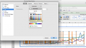
At this point, you can right click on the series again, select “Format Data Series…”, and change the Fill color to a light gray.
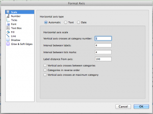
Next, we tell the x axis what the correct labels are (the “Year” column) and have the labels show up every 4 years. (Our data series start on an election year, so the labels will always appear on election years.)
- Right click inside the chart somewhere and select “Select Data…”
- Select any of the data series in the “Series” list, then go over to the “Category (X) axis labels” box and select the “Year” column. Click “OK”.

- Right-click on the x axis and select “Format Axis…”.
- Under “Scale”:
- Under “Text Box”, select the text direction of “Rotate to 90 deg Counterclockwise”. Click “OK”.

The x axis should have appropriate year labels now. The y axis can similarly be adjusted to show just the range of values we’re most interested in.
The rest of the changes are simply formatting changes. Right-click on the individual data series to change the colors, line widths, etc. Use the formatting options or the Chart tools on the Excel ribbon to change the font of any text, adjust the grid lines, add labels and titles, etc. The data series names in the legend can be adjusted by using the “Select Data…” option and typing in custom text in the “Name” field.
The final product should have colored regions and look something like the chart below.
In another post, we will show how to spice this chart up even more using Adobe Illustrator.


