All posts by Noah Huffman

Auditing Archival Description for Harmful Language: A Computer and Community Effort

This post was written by Miriam Shams-Rainey, a third-year undergraduate at Duke studying Computer Science and Linguistics with a minor in Arabic. As a student employee in the Rubenstein’s Technical Services Department in the Summer of 2021, Miriam helped build a tool to audit archival description in the Rubenstein for potentially harmful language. In this post, she summarizes her work on that project.

The Rubenstein Library has collections ranging across centuries. Its collections are massive and often contain rare manuscripts or one of a kind data. However, with this wide-ranging history often comes language that is dated, harmful, often racist, sexist, homophobic, and/or colonialist. As important as it is to find and remediate these instances of potentially harmful language, there is lot of data that must be searched.

With over 4,000 collection guides (finding aids) and roughly 12,000 catalog records describing archival collections, archivists would need to spend months of time combing their metadata to find harmful or problematic language before even starting to find ways to handle this language. That is, unless there was a way to optimize this workflow.

Working under Noah Huffman’s direction and the imperatives of the Duke Libraries’ Anti-Racist Roadmap, I developed a Python program capable of finding occurrences of potentially harmful language in library metadata and recording them for manual analysis and remediation. What would have taken months of work can now be done in a few button clicks and ten minutes of processing time. Moreover, the tools I have developed are accessible to any interested parties via a GitHub repository to modify or expand upon.

Although these gains in speed push metadata language remediation efforts at the Rubenstein forward significantly, a computer can only take this process so far; once uses of this language have been identified, the responsibility of determining the impact of the term in context falls onto archivists and the communities their work represents. To this end, I have also outlined categories of harmful language occurrences to act as a starting point for archivists to better understand the harmful narratives their data uphold and developed best practices to dismantle them.

Building an automated audit tool
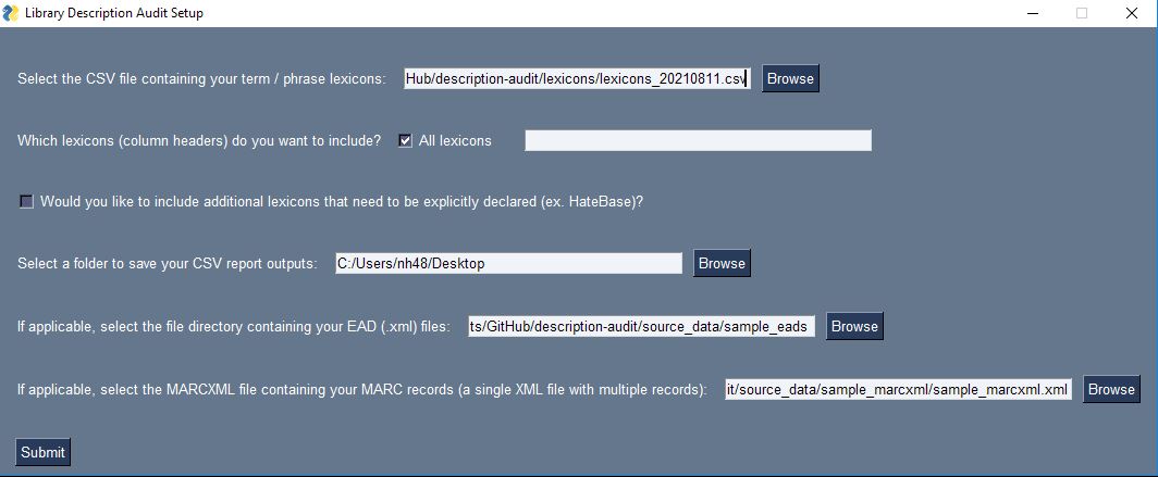
Audit Tool GUI Screenshot
The simple, yet user-friendly interface that allows archivists to customize the search audit to their specific needs.

I created an executable that allows users to interact with the program regardless of their familiarity with Python or with using their computer’s command line. With an executable, all that a user must do is simply click on the program (titled “description_audit.exe”) and the script will load with all of its dependencies in a self-contained environment. There’s nothing that a user needs to install, not even Python.

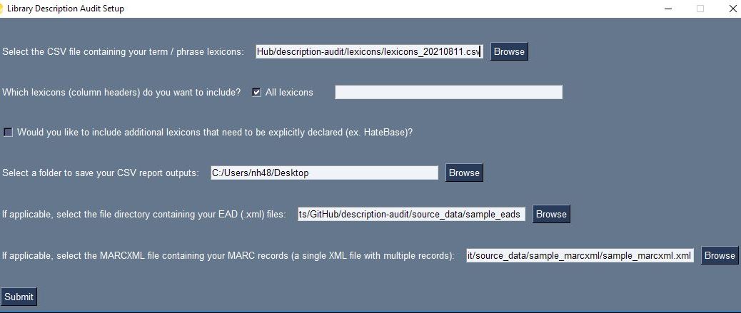
Within this executable, I also created a user interface to allow users to set up the program with their specific audit parameters. To use this program, users should first create a CSV file (spreadsheet) containing each list of words they want to look for in their metadata.
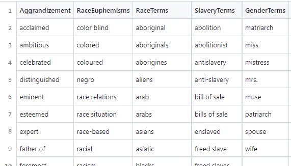
Snippet of Lexicon CSV
Snippet from a sample lexicon CSV file containing harmful terms to search

In this CSV file of “lexicons”, each category of terms  should have its own column, for example RaceTerms could be the first row in a column of terms such as “colored” or “negro,” and GenderTerms could be the first row in a column of gendered terms such as “homemaker” or “wife.”  See these lexicon CSV file examples.

Once this CSV has been created, users can select this CSV of lexicons in the program’s user interface and then select which columns of terms they want the program to use when searching across the source metadata. Users can either use all lexicon categories (all columns) by default or specify a subset by typing out those column headers. For the Rubenstein’s purposes, there is also a rather long lexicon called HateBase (from a regional, multilingual database of potential hate speech terms often used in online moderating) that is only enabled when a checkbox is checked; users from other institutions can download the HateBase lexicon for themselves and use it or they can simply ignore it.

In the CSV reports that are output by the program, matches for harmful terms and phrases will be tagged with the specific lexicon category the match came from, allowing users to filter results to certain categories of potentially harmful terms.

Users also need to designate a folder on their desktop where report outputs should be stored, along with the folder containing their source EAD records in .xml format and their source MARCXML file containing all of the MARC records they wish to process as a single XML file. Results from MARC and EAD records are reported separately, so only one type of record is required to use the program, however both can be provided in the same session.

How archival metadata is parsed and analyzed

Once users submit their input parameters in the GUI, the program begins by accessing the specified lexicons from the given CSV file. For each lexicon, a “rule” is created for a SpaCy rule-based matcher, using the column name (e.g. RaceTerms or GenderTerms) as the name of the specific rule. The same SpaCy matcher object identifies matches to each of the several lexicons or “rules”. Once the matcher has been configured, the program assesses whether valid MARC or EAD records were given and starts reading in their data.

To access important pieces of data from each of these records, I used a Python library called BeautifulSoup to parse the XML files. For each individual record, the program parses the call numbers and collection or entry name so that information can be included in the CSV reports. For EAD records, the collection title and component titles  are also parsed to be analyzed for matches to the lexicons, along with any data that is in a paragraph (<p>) tag. For MARC records, the program also parses the author or creator of the item, the extent of the collection, and the timestamp of when the description of the item was last updated. In each MARC record, the 520 field (summary)  and 545 field (biography/history note) are all concatenated together and analyzed as a single entity.

Data from each record is stored in a Python dictionary with the names of fields (as strings) as keys mapping to the collection title, call number, etc. Each of these dictionaries is stored in a list, with a separate structure for EAD and MARC records.

Once data has been parsed and stored, each record is checked for matches to the given lexicons using the SpaCy rule-based matcher. For each record, any matches that are found are then stored in the dictionary with the matching term, the context of the term (the entire field or surrounding few sentences, depending on length), and the rule the term matches (such as RaceTerms). These matches are found using simple tokenization from SpaCy that allow matches to be identified quickly and without regard for punctuation, capitalization, etc. 

Although this process doesn’t necessarily use the cutting-edge of natural language processing that the SpaCy library makes accessible, this process is adaptable in ways that matching procedures like using regular expressions often isn’t. Moreover, identifying and remedying harmful language is a fundamentally human process which, at the end of the day, needs a significant level of input both from historically marginalized communities and from archivists.

Matches to any of the lexicons, along with all other associated data (the record’s call number, title, etc.) are then written into CSV files for further analysis and further categorization by users. You can see sample CSV audit reports here. The second phase of manual categorization is still a lengthy process, yielding roughly 14600 matches from the Rubenstein Library’s EAD data and 4600 from its MARC data which must still be read through and analyzed by hand, but the process of identifying these matches has been computerized to take a mere ten minutes, where it could otherwise be a months-long process.

Categorizing matches: an archivist and community effort
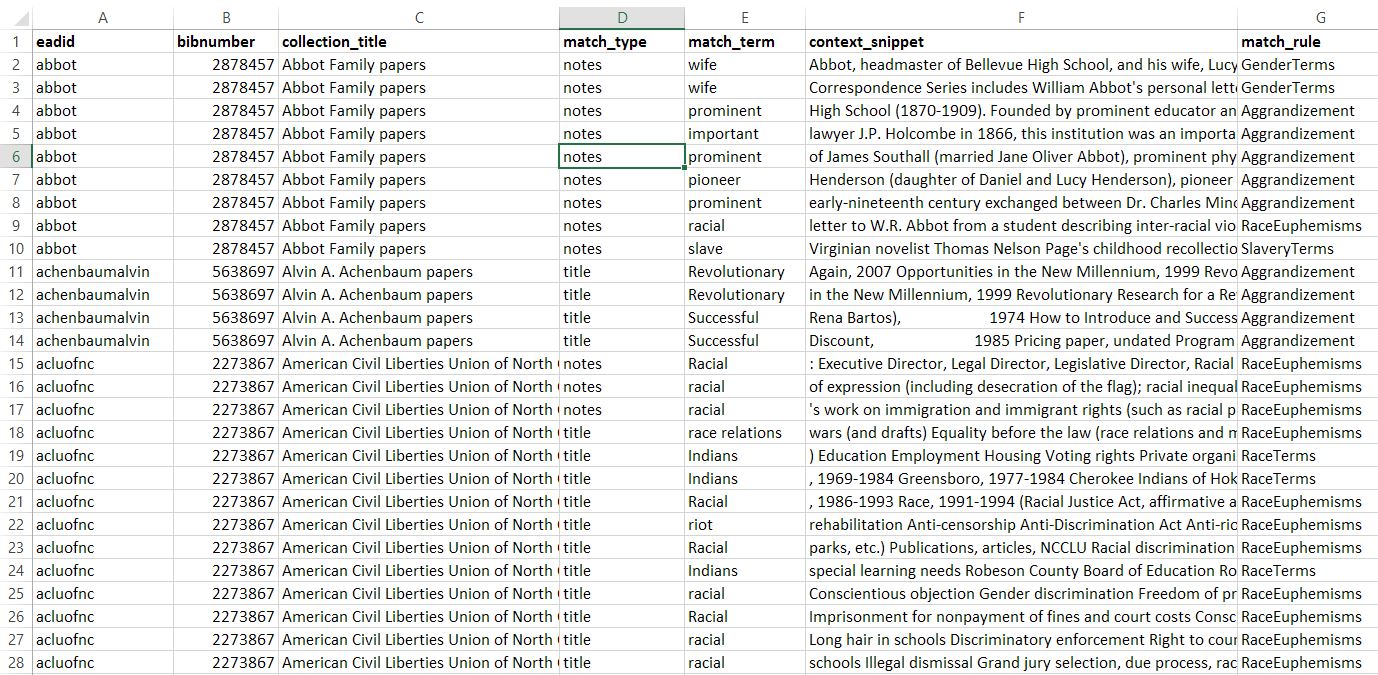
An excerpt of initial data returned by the audit program for EAD records. This data should be further categorized manually to ensure a comprehensive and nuanced understanding of these instances of potentially harmful language.

To better understand these matches and create a strategy to remediate the harmful language they represent, it is important to consider each match in several different facets.

Looking at the context provided with each match allows archivists to understand the way in which the term was used. The remediation strategy for the use of a potentially harmful term in a proper noun used as a positive, self-identifying term, such as the National Association for the Advancement of Colored People, for example, is vastly different from that of a white person using the word “colored” as a racist insult.

The three ways in which I proposed we evaluate context are as follows:

  1. Match speaker: who was using the term? Was the sensitive term being used as a form of self-identification or reclaiming by members of a marginalized group, was it being used by an archivist, or was it used by someone with privilege over the marginalized group the term targets (e.g. a white person using an anti-Black term or a cisgender straight person using an anti-LGBTQ+ term)? Within this category, I proposed three potential categories for uses of a term: in-group, out-group, and archivist. If a term is used by a member (or members) of the identity group it references, its use is considered an in-group use. If the term is used by someone who is not a member of the identity group the term references, that usage of the term is considered out-group. Paraphrasing or dated term use by archivists is designated simply as archivist use.
  2. Match context: how was the term in question being used? Modifying the text used in a direct quote or a proper noun constitutes a far greater liberty by the archivist than removing a paraphrased section or completely archivist-written section of text that involved harmful language. Although this category is likely to evolve as more matches are categorized, my initial proposed categories are: proper noun, direct quote, paraphrasing, and archivist narrative.
  3. Match impact: what was the impact of the term? Was this instance a false positive, wherein the use of the term was in a completely unrelated and innocuous context (e.g. the use of the word “colored” to describe the colors used in visual media), or was the use of the term in fact harmful? Was the use of the term derogatory, or was it merely a mention of politicized identities? In many ways, determining the impact of a particular term or use of potentially harmful language is a community effort; if a community member with a marginalized identity says that the use of a term in that particular context is harmful to people with that identity, archivists are in no position to disagree or invalidate those feelings and experiences. The categories that I’ve laid out initially–dated original term, dated Rubenstein term, mention of marginalized issues, mention of marginalized identity, downplaying bias (e.g. calling racism and discrimination an issue with “race relations”), dehumanization of marginalized people, false positive–only hope to serve as an entry point and rudimentary categorization of these nuances to begin this process.
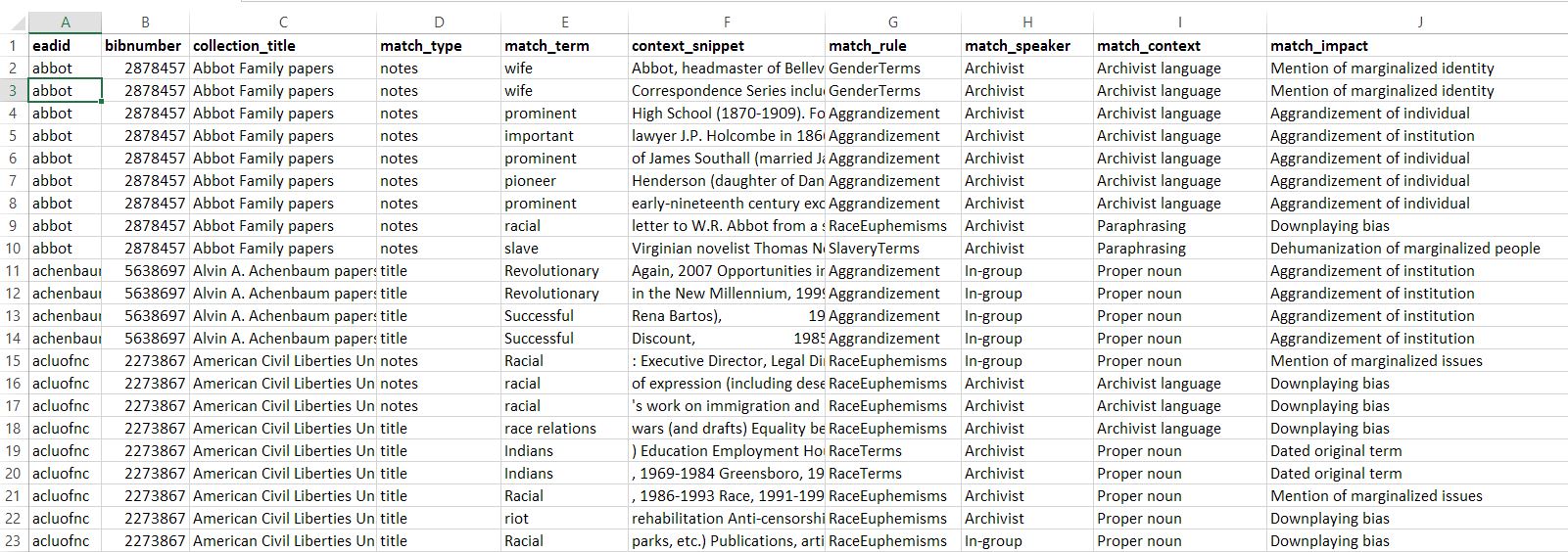
A short excerpt of categorized EAD metadata

Here you can find more documentation on the manual categorization strategy.

Categorizing each of these instances of potentially harmful language remains a time-consuming, meticulous process. Although much of this work can be computerized, decolonization is a fundamentally human and fundamentally community-centered practice. No computer can dismantle the colonial, white supremacist narratives that archival work often upholds. This work requires our full attention and, for better or for worse, a lot of time, even with the productivity boost technology gives us.

Once categories have been established, at least on a preliminary level, I found that about 100-200 instances of potentially harmful language could be manually parsed and categorized in an hour.

Conclusion

Decolonization and anti-racist efforts in archival work are an ongoing process. It is bound to take active learning, reflection, and lots of remediation. However, using technology to start this process creates a much less daunting entry point. Anti-racism work is essential in archival spaces.

The ways we talk about history can either work to uphold traditional white supremacist, racist, ableist, etc. narratives, or they can work to dismantle them. In many ways, archival work has often upheld these narratives in the past, however this audit represents the sincere beginnings of work to further equitable narratives in the future.

“To Greenland in 105 Days, or, Why Did I Ever Leave Home”: Henry J. Oosting’s Misadventure in the Arctic (1937)

When Duke professor and botanist Henry J. Oosting agreed to take part in an expedition to Greenland in the summer of 1937 his mission was to collect botanical samples and document the region’s native flora. The expedition, organized and led by noted polar explorer Louise Arner Boyd, included several other accomplished scientists of the day and its principal achievement was the discovery and charting of a submarine ridge off of Greenland’s eastern coast.

Narwhal sketch
Oosting’s sketch of a Narwhal

In a diary he kept during his trip titled “To Greenland in 105 Days, or Why did I ever leave home,” Oosting focuses little on the expedition’s scientific exploits. Instead, he offers a more intimate look into the mundane and, at times, amusing aspects of early polar exploration. Supplementing the diary in the recently published Henry J. Oosting papers digital collection are a handful of digitized nitrate negatives that add visual interest to his arctic (mis)adventures.

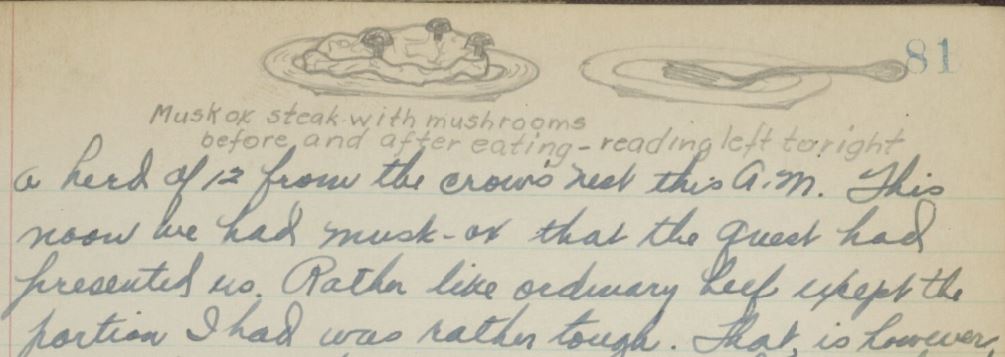
Oosting’s journey got off to an inauspicious start when he wrote in his opening entry on June 9, 1937: “Frankly, I’m not particularly anxious to go now that the time has come–adventure of any sort has never been my line–and the thought of the rolling sea gives me no great cheer.” What follows over the next 200 pages or so, by his own account, are the “inane mental ramblings of a simple-minded botanist,” complete with dozens of equally inane marginal doodles.

Musk Ox Steak doodle
Oosting sketch of Musk Ox steak

The Veslekari, the ship chartered by Louise Boyd for the expedition, first encountered sea ice on July 12 just off the east coast of Greenland. As the ship slowed to a crawl and boredom set in among the crew the following day, Oosting wrote in his diary that “Miss Boyd’s story of the polar bear is worth recording.” He then relayed a joke Boyd told the crew: “If you keep a private school and I keep a private school then why does a polar bear sit on a cake of ice…? To keep its privates cool, of course.”  For clarification, Oosting added: “She says she has been trying for a long time to get just the right picture to illustrate the story but it’s either the wrong kind of bear or it won’t hold its position.”

Hoisting a polar bear
Crew hoisting a polar bear on board the Veslekari

When the expedition finally reached the Greenland coast at the end of July, Oosting spent several days exploring the Tyrolerfjord glacier, gathering plant specimens and drying them on racks in the ship’s engine room. On the glacier, Oosting observed an arctic hare, an ermine, and noted that “my plants are accumulating in such quantity.”

Oosting sketch of foot

As the expedition wore on Oosting grew increasingly frustrated with the daily tedium and with Boyd’s unfailing enthusiasm for the enterprise. “In spite of everything…we are stopping at more or less regular intervals to see what B thinks is interesting,” Oosting wrote on August 19.  “I didn’t go ashore this A.M. for a 15 min. stop even after she suggested it–have heard about it 10 times since…I’ll be obliged to go in every time now regardless or there will be no living with this woman. I am thankful, sincerely thankful, there are only 5 more days before we sail for I am thoroughly fed-up with this whole business.”

Arctic Hare
Arctic Hare

By late August, the Veslekari and crew headed back east towards Bergen, Norway and eventually Newcastle, England, where Oosting boarded a train for London on September 12. “This sleeping car is the silliest arrangement imaginable,” Oosting wrote, “my opinion of the English has gone down–at least my opinion of their ideas of comfort.” After a brief stint sightseeing around London, Oosting boarded another ship in Southampton headed for New York and eventually home to Durham. “It will be heaven to get back to the peace and quiet of Durham,” Oosting pined on September 14, “I’m developing a soft spot for the lousy old town.”

Veslekari
Veslekari, the vessel chartered by Louise Boyd for the 1937 Greenland expedition

Oosting arrived home on September 21, where his diary ends. Despite his curmudgeonly tone throughout and his obsession with recording every inconvenience and impediment encountered along the way, it’s clear from other sources that Oosting’s work on the voyage made important contributions to our understanding of arctic plant life.

In The Coast of Northeast Greenland (1948), edited by Louise Boyd and published by the American Geographic Society, Oosting authored a chapter titled “Ecological Notes on the Flora,” in which he meticulously documented the specimens he collected in the arctic. The onset of World War II and concerns over national security delayed publication of Oosting’s findings, but when released, they provided valuable new information about plant communities in the region.  While Oosting’s diary reveals a man with little appetite for adventure, his work endures.  As the forward to Boyd’s 1948 volume attests:  “When travelers can include significant contributions to science, then adventure becomes a notable achievement.”

Oosting sketch
Oosting sketch

Getting Things Done in ArchivesSpace, or, Fun with APIs

aspace_iconMy work involves a lot of problem-solving and problem solving often requires learning new skills. It’s one of the things I like most about my job. Over the past year, I’ve spent most of my time helping Duke’s Rubenstein Library implement ArchivesSpace, an open source web application for managing information about archival collections.

As an archivist and metadata librarian by training (translation: not a programmer), I’ve been working mostly on data mapping and migration tasks, but part of my deep-dive into ArchivesSpace has been learning about the ArchivesSpace API, or, really, learning about APIs in general–how they work, and how to take advantage of them. In particular, I’ve been trying to find ways we can use the ArchivesSpace API to work smarter and not harder as the saying goes.

Why use the ArchivesSpace API?

Quite simply, the ArchivesSpace API lets you do things you can’t do in the staff interface of the application, especially batch operations.

So what is the ArchivesSpace API? In very simple terms, it is a way to interact with the ArchivesSpace backend without using the application interface. To learn more, you should check out this excellent post from the University of Michigan’s Bentley Historical Library: The ArchivesSpace API.

aspace_api_doc_example
Screenshot of ArchivesSpace API documentation showing how to form a GET request for an archival object record using the “find_by_id” endpoint

Working with the ArchivesSpace API: Other stuff you might need to know

As with any new technology, it’s hard to learn about APIs in isolation. Figuring out how to work with the ArchivesSpace API has introduced me to a suite of other technologies–the Python programming language, data structure standards like JSON, something called cURL, and even GitHub.  These are all technologies I’ve wanted to learn at some point in time, but I’ve always found it difficult to block out time to explore them without having a concrete problem to solve.

Fortunately (I guess?), ArchivesSpace gave me some concrete problems–lots of them.  These problems usually surface when a colleague asks me to perform some kind of batch operation in ArchivesSpace (e.g. export a batch of EAD, update a bunch of URLs, or add a note to a batch of records).

Below are examples of some of the requests I’ve received and some links to scripts and other tools (on Github) that I developed for solving these problems using the ArchivesSpace API.

ArchivesSpace API examples:

“Can you re-publish these 12 finding aids again because I fixed some typos?”

Problem:

I get this request all the time. To publish finding aids at Duke, we export EAD from ArchivesSpace and post it to a webserver where various stylesheets and scripts help render the XML in our public finding aid interface. Exporting EAD from the ArchivesSpace staff interface is fairly labor intensive. It involves logging into the application, finding the collection record (resource record in ASpace-speak) you want to export, opening the record, making sure the resource record and all of its components are marked “published,” clicking the export button, and then specifying the export options, filename, and file path where you want to save the XML.

In addition to this long list of steps, the ArchivesSpace EAD export service is really slow, with large finding aids often taking 5-10 minutes to export completely. If you need to post several EADs at once, this entire process could take hours–exporting the record, waiting for the export to finish, and then following the steps again.  A few weeks after we went into production with ArchivesSpace I found that I was spending WAY TOO MUCH TIME exporting and re-exporting EAD from ArchivesSpace. There had to be a better way…

Solution:

asEADpublish_and_export_eadid_input.py – A Python script that batch exports EAD from the ArchivesSpace API based on EADID input. Run from the command line, the script prompts for a list of EADID values separated with commas and checks to see if a resource record’s finding aid status is set to ‘published’. If so, it exports the EAD to a specified location using the EADID as the filename. If it’s not set to ‘published,’ the script updates the finding aid status to ‘published’ and then publishes the resource record and all its components. Then, it exports the modified EAD. See comments in the script for more details.

Below is a screenshot of the script in action. It even prints out some useful information to the terminal (filename | collection number | ASpace record URI | last person to modify | last modified date | export confirmation)

EAD Batch Export Script
Terminal output from EAD batch export script

[Note that there are some other nice solutions for batch exporting EAD from ArchivesSpace, namely the ArchivesSpace-Export-Service plugin.]

“Can you update the URLs for all the digital objects in this collection?”

Problem:

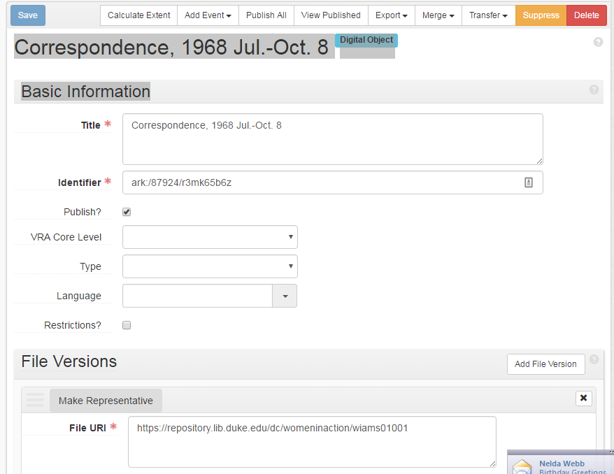
We’re migrating most of our digitized content to the new Duke Digital Repository (DDR) and in the process our digital objects are getting new (and hopefully more persistent) URIs. To avoid broken links in our finding aids to digital objects stored in the DDR, we need to update several thousand digital object URLs in ArchivesSpace that point to old locations. Changing the URLs one at a time in the ArchivesSpace staff interface would take, you guessed it, WAY TOO MUCH TIME.  While there are probably other ways to change the URLs in batch (SQL updates?), I decided the safest way was to, of course, use the ArchivesSpace API.

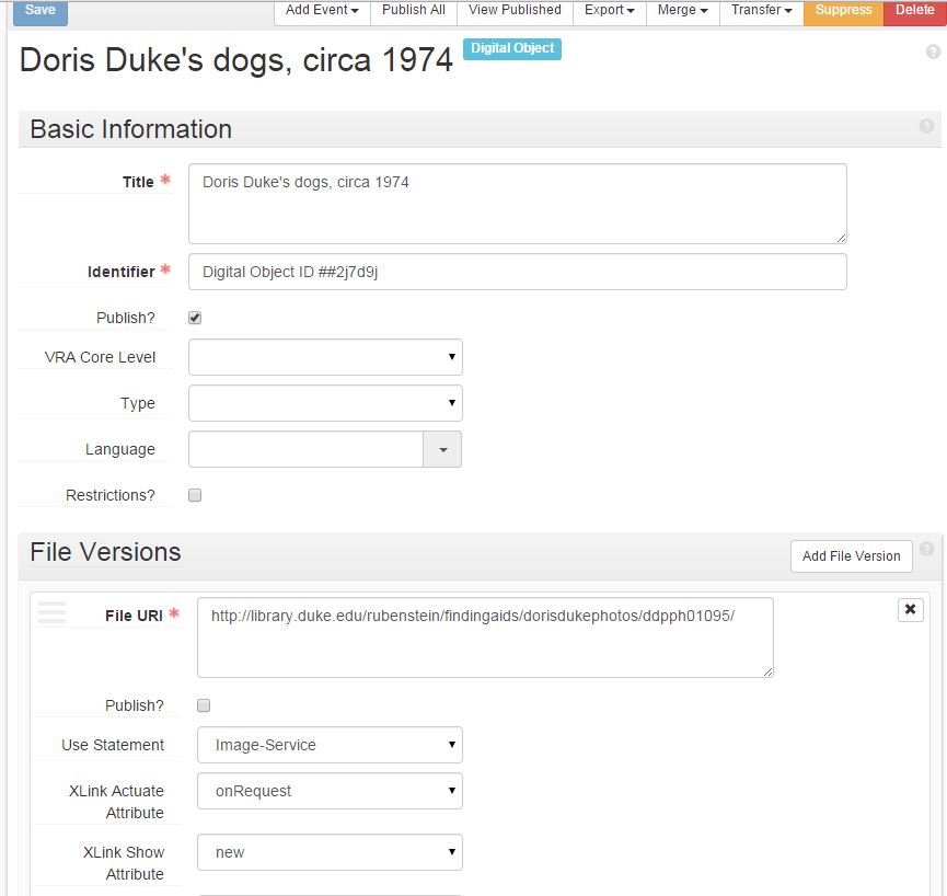
Digital Object Screenshot
Screenshot of a Digital Object record in ArchivesSpace. The asUpdateDAOs.py script will batch update identifiers and file version URIs based on an input CSV
Solution:

asUpdateDAOs.py – A Python script that will batch update Digital Object identifiers and file version URIs in ArchivesSpace based on an input CSV file that contains refIDs for the the linked Archival Object records. The input is a five column CSV file (without column headers) that includes: [old file version use statement], [old file version URI], [new file version URI], [ASpace ref_id], [ark identifier in DDR (e.g. ark:/87924/r34j0b091)].

[WARNING: The script above only works for ArchivesSpace version 1.5.0 and later because it uses the new “find_by_id” endpoint. The script is also highly customized for our environment, but could easily be modified to make other batch changes to digital object records based on CSV input. I’d recommend testing this in a development environment before using in production].

“Can you add a note to these 300 records?”

Problem:

We often need to add a note or some other bit of metadata to a set of resource records or component records in ArchivesSpace. As you’ve probably learned, making these kinds of batch updates isn’t really possible through the ArchivesSpace staff interface, but you can do it using the ArchivesSpace API!

Solution:

duke_archival_object_metadata_adder.py –  A Python script that reads a CSV input file and batch adds ‘repository processing notes’ to archival object records in ArchivesSpace. The input is a simple two-column CSV file (without column headers) where the first column contains the archival object’s ref_ID and the second column contains the text of the note you want to add. You could easily modify this script to batch add metadata to other fields.

duke_archival_object_metadata_adder
Terminal output of duke_archival_object_metadata_adder.py script

[WARNING: Script only works in ArchivesSpace version 1.5.0 and higher].

Conclusion

The ArchivesSpace API is a really powerful tool for getting stuff done in ArchivesSpace. Having an open API is one of the real benefits of an open-source tool like ArchivesSpace. The API enables the community of ArchivesSpace users to develop their own solutions to local problems without having to rely on a central developer or development team.

There is already a healthy ecosystem of ArchivesSpace users who have shared their API tips and tricks with the community. I’d like to thank all of them for sharing their expertise, and more importantly, their example scripts and documentation.

Here are more resources for exploring the ArchivesSpace API:

Baby Steps towards Metadata Synchronization

How We Got Here: A terribly simplistic history of library metadata

Managing the description of library collections (especially “special” collections) is an increasingly complex task.  In the days of yore, we bought books and other things, typed up or purchased catalog cards describing those things (metadata), and filed the cards away.  It was tedious work, but fairly straightforward.  If you wanted to know something about anything in the library’s collection, you went to the card catalog.  Simple.

Some time in the 1970s or 1980s we migrated all (well, most) of that card catalog description to the ILS (Integrated Library System).  If you wanted to describe something in the library, you made a MARC record in the ILS.  Patrons searched those MARC records in the OPAC (the public-facing view of the ILS).  Still pretty simple.  Sure, we maintained other paper-based tools for managing description of manuscript and archival collections (printed finding aids, registers, etc.), but until somewhat recently, the ILS was really the only “system” in use in the library.

duke_online_catalog_1980s
Duke Online Catalog, 1980s

From the 1990s on things got complicated. We started making EAD and MARC records for archival collections. We started digitizing parts of those collections and creating Dublin Core records and sometimes TEI for the digital objects.  We created and stored library metadata in relational databases (MySQL), METS, MODS, and even flat HTML. As library metadata standards proliferated, so too did the systems we used the create, manage, and store that metadata.

Now, we have an ILS for managing MARC-based catalog records, ArchivesSpace for managing more detailed descriptions of manuscript collections, a Fedora (Hydra) repository for managing digital objects, CONTENTdm for managing some other digital objects, and lots of little intermediary descriptive tools (spreadsheets, databases, etc.).  Each of these systems stores library metadata in a different format and in varying levels of detail.

So what’s the problem and what are we doing about it?

The variety of metadata standards and systems isn’t the problem.  What is the problem–a very painful and time-consuming problem–is having to maintain and reconcile description of the same thing (a manuscript, a folder of letters, an image, an audio file, etc.) across all these disparate metadata formats and systems.  It’s a metadata synchronization problem and it’s a big one.

For the past four months or so, a group of archivists and developers here in the library have been meeting regularly to brainstorm ways to solve or at least help alleviate some of our metadata synchronization problems.  We’ve been calling our group “The Synchronizers.”

What have The Synchronizers been up to?  Well, so far we’ve been trying to tackle two pieces of the synchronization conundrum:

Problem 1 (the big one): Keeping metadata for special collections materials in sync across ArchivesSpace, the digitization process, and our Hydra repository.

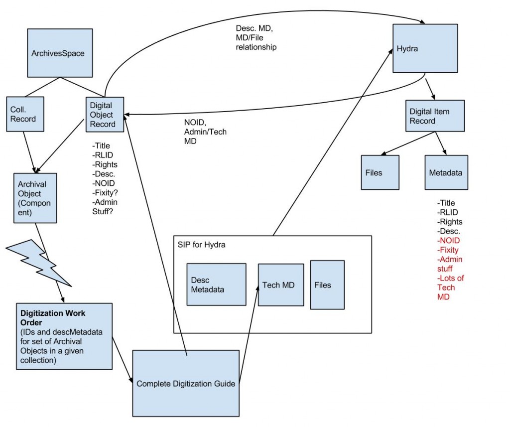
Ideally, we’d like to re-purpose metadata from ArchivesSpace to facilitate the digitization process and also keep that metadata in sync as items are digitized, described more fully, and ingested into our Hydra repository. Fortunately, we’re not the only library trying to tackle this problem.  For more on AS/Hydra integration, see the work of the Hydra Archivists Interest Group.

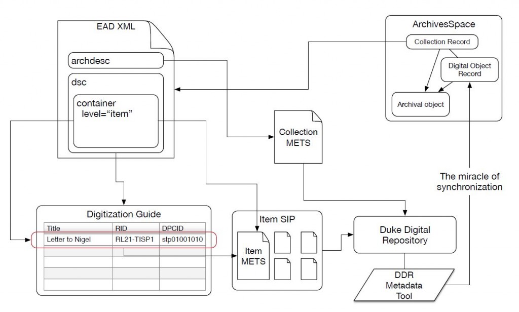
Below are a couple of rough sketches we drafted to start thinking about this problem at Duke.

AS_Hydra_diagram
Hydra / ArchivesSpace Integration Sketch, take 1
sychronizers_will
Hydra / ArchivesSpace Integration Sketch, take 2


In addition to these systems integration diagrams, I’ve been working on some basic tools (scripts) that address two small pieces of this larger problem:

  • A script to auto-generate digitization guides by extracting metadata from ArchivesSpace-generated EAD files (digitization guides are simply spreadsheets we use to keep track of what we digitize and to assign identifiers to digital objects and files during the digitization process).
  • A script that uses a completed digitization guide to batch-create digital object records in ArchivesSpace and at the same time link those digital objects to the descriptions of the physical items (the archival object records in ArchivesSpace-speak).  Special thanks to Dallas Pillen at the University of Michigan for doing most of the heavy lifting on this script.

Problem 2 (the smaller one): Using ArchivesSpace to produce MARC records for archival collections (or, stopping all that cutting and pasting).

In the past, we’ve had two completely separate workflows in special collections for creating archival description in EAD and creating collection-level MARC records for those same collections.  Archivists churned out detailed EAD finding aids and catalogers took those finding aids, and cut-and-pasted relevant sections into collection-level MARC records.  It’s quite silly, really, and we need a better solution that saves time and keeps metadata consistent across platforms.

While we haven’t done much work in this area yet, we have formed a small working group of archivists/catalogers and developed the following work plan:

  1. Examine default ArchivesSpace MARC exports and compare those exports to current MARC cataloging practices (document differences).
  2. Examine differences between ArchivesSpace MARC and “native” MARC and decide which current practices are worth maintaining keeping in mind we’ll need to modify default ArchivesSpace MARC exports to meet current MARC authoring practices.
  3. Develop cross-walking scripts or modify the ArchivesSpace MARC exporter to generate usable MARC data from ArchivesSpace.
  4. Develop and document an efficient workflow for pushing or harvesting MARC data from ArchivesSpace to both OCLC and our local ILS.
  5. If possible, develop, test, and document tools and workflows for re-purposing container (instance) information in ArchivesSpace in order to batch-create item records in the ILS for archival containers (boxes, folders, etc).
  6. Develop training for staff on new ArchivesSpace to MARC workflows.
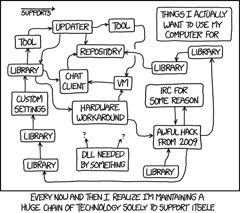
courtesy of xkcd.com

Conclusion

So far we’ve only taken baby steps towards our dream of TOTAL METADATA SYNCHRONIZATION, but we’re making progress.  Please let us know if you’re working on similar projects at your institution. We’d love to hear from you.

The Tao of the DAO: Embedding digital objects in finding aids

Over the last few months, we’ve been doing some behind-the-scenes re-engineering of “the way” we publish digital objects in finding aids (aka “collection guides”).  We made these changes in response to two main developments:

  • The transition to ArchivesSpace for managing description of archival collections and the production of finding aids
  • A growing need to handle new types, or classes, of digital objects in our finding aid interface (especially born-digital electronic records)

Background

While the majority of items found in Duke Digital Collections are published and accessible through our primary digital collections interface (codename Tripod), we have a growing number of digital objects that are published (and sometimes embedded) in finding aids.

Finding aids describe the contents of manuscript and archival collections, and in many cases, we’ve digitized all or portions of these collections.  Some collections may contain material that we acquired in digital form.  For a variety of reasons that I won’t describe here, we’ve decided that embedding digital objects directly in finding aids can be a suitable, often low-barrier alternative to publishing them in our primary digital collections platform.  You can read more on that decision here.

ahstephens_screenshot
Screenshot showing digital objects embedded in the Alexander H. Stephens Papers finding aid


EAD, ArchivesSpace, and the <dao>

At Duke, we’ve been creating finding aids in EAD (Encoded Archival Description) since the late 1990s.  Prior to implementing ArchivesSpace (June 2015) and its predecessor Archivists Toolkit (2012), we created EAD through some combination of an XML editor (NoteTab, Oxygen), Excel spreadsheets, custom scripts, templates, and macros.  Not surprisingly, the evolution of EAD authoring tools led to a good deal of inconsistent encoding across our EAD corpus.  These inconsistencies were particularly apparent when it came to information encoded in the <dao> element, the EAD element used to describe “digital archival objects” in a collection.

As part of our ArchivesSpace implementation plan, we decided to get better control over the <dao>–both its content and its structure.  We wrote some local best practice guidelines for formatting the data contained in the <dao> element and we wrote some scripts to normalize our existing data before migrating it to ArchivesSpace.

Classifying digital objects with the “use statement.”

In June 2015, we migrated all of our finding aids and other descriptive data to ArchivesSpace.  In total, we now have about 3400 finding aids (resource records) and over 9,000 associated digital objects described in ArchivesSpace.  Among these 9,000 digital objects, there are high-res master images, low-res use copies, audio files, video files, disk image files, and many other kinds of digital content.  Further, the digital files are stored in several different locations–some accessible to the public and some restricted to staff.

In order for our finding aid interface to display each type of digital object properly, we developed a classification system of sorts that 1) clearly identifies each class of digital object and 2) describes the desired display behavior for that type of object in our finding aid interface.

In ArchivesSpace, we store that information consistently in the ‘Use Statement’ field of each Digital Object record.  We’ve developed a core set of use statement values that we can easily maintain in a controlled value list in the ArchivesSpace application.  In turn, when ArchivesSpace generates or exports an EAD file for any given collection that contains digital objects, these use statement values are output in the DAO role attribute.  Actually, a minor bug in the ArchivesSpace application currently prevents the use statement information from appearing in the <dao>. I fixed this by customizing the ArchivesSpace EAD serializer in a local plugin.

file_version_aspace_example
Screenshot from ArchivesSpace showing digital object record, file version, and use statement


duke_dao_code
Snippet of EAD generated from ArchivesSpace showing <dao> encoding

 Every object its viewer/player

The values in the DAO role attribute tell our display interface how to render a digital object in the finding aid.  For example, when the display interface encounters a DAO with role=”video-streaming” it knows to queue up our embedded streaming video player.  We have custom viewers and players for audio, batches of image files, PDFs, and many other content types.

Here are links to some finding aids with different classes of embedded digital objects, each with its own associated use statement and viewer/player.

The curious case of electronic records

The last example above illustrates the curious case of electronic records.  The term “electronic records” can describe a wide range of materials but may include things like email archives, disk images, and other formats that are not immediately accessible on our website, but must be used by patrons in the reading room on a secure machine.  In these cases, we want to store information about these files in ArchivesSpace and provide a convenient way for patrons to request access to them in the finding aid interface.

Within the next few weeks, we plan to implement some improvements to the way we handle the description of and access to electronic records in finding aids.  Eventually, patrons will be able to view detailed information about the electronic records by hovering over a link in the finding aid.  Clicking on the link will automatically generate a request for those records in Aeon, the Rubenstein Library’s request management system.  Staff can then review and process those requests and, if necessary, prepare the electronic records for viewing on the reading room desktop.

Conclusion

While we continue to tweak our finding aid interface and learn our way around ArchivesSpace, we think we’ve developed a fairly sustainable and flexible way to publish digital objects in finding aids that both preserves the archival context of the items and provides an engaging user-experience for interacting with the objects.  As always, we’d love to hear how other libraries may have tackled this same problem.  Please share your comments or experiences with handling digital objects in finding aids!

[Credit to Lynn Holdzkom at UNC-Chapel Hill for coining the phrase “The Tao of the DAO”]

Adventures in metadata hygiene: using Open Refine, XSLT, and Excel to dedup and reconcile name and subject headings in EAD

OpenRefine, formerly Google Refine, bills itself as “a free, open source, powerful tool for working with messy data.”  As someone who works with messy data almost every day, I can’t recommend it enough.  While Open Refine is a great tool for cleaning up “grid-shaped data” (spreadsheets), it’s a bit more challenging to use when your source data is in some other format, particularly XML.

Some corporate name terms from an EAD collection guide
Some corporate name terms from an EAD (XML) collection guide

As part of a recent project to migrate data from EAD (Encoded Archival Description) to ArchivesSpace, I needed to clean up about 27,000 name and subject headings spread across over 2,000 EAD records in XML.  Because the majority of these EAD XML files were encoded by hand using a basic text editor (don’t ask why), I knew there were likely to be variants of the same subject and name terms throughout the corpus–terms with extra white space, different punctuation and capitalization, etc.  I needed a quick way to analyze all these terms, dedup them, normalize them, and update the XML before importing it into ArchivesSpace.  I knew Open Refine was the tool for the job, but the process of getting the terms 1) out of the EAD, 2) into OpenRefine for munging, and 3) back into EAD wasn’t something I’d tackled before.

Below is a basic outline of the workflow I devised, combining XSLT, OpenRefine, and, yes, Excel.  I’ve provided links to some source files when available.  As with any major data cleanup project, I’m sure there are 100 better ways to do this, but hopefully somebody will find something useful here.

1. Use XSLT to extract names and subjects from EAD files into a spreadsheet

I’ve said it before, but sooner or later all metadata is a spreadsheet. Here is some XSLT that will extract all the subjects, names, places and genre terms from the <controlaccess> section in a directory full of EAD files and then dump those terms along with some other information into a tab-separated spreadsheet with four columns: original_term, cleaned_term (empty), term_type, and eadid_term_source.

controlaccess_extractor.xsl

 2. Import the spreadsheet into OpenRefine and clean the messy data!

Once you open the resulting tab delimited file in OpenRefine, you’ll see the four columns of data above, with “cleaned_term” column empty. Copy the values from the first column (original_term) to the second column (cleaned_term).  You’ll want to preserve the original terms in the first column and only edit the terms in the second column so you can have a way to match the old values in your EAD with any edited values later on.

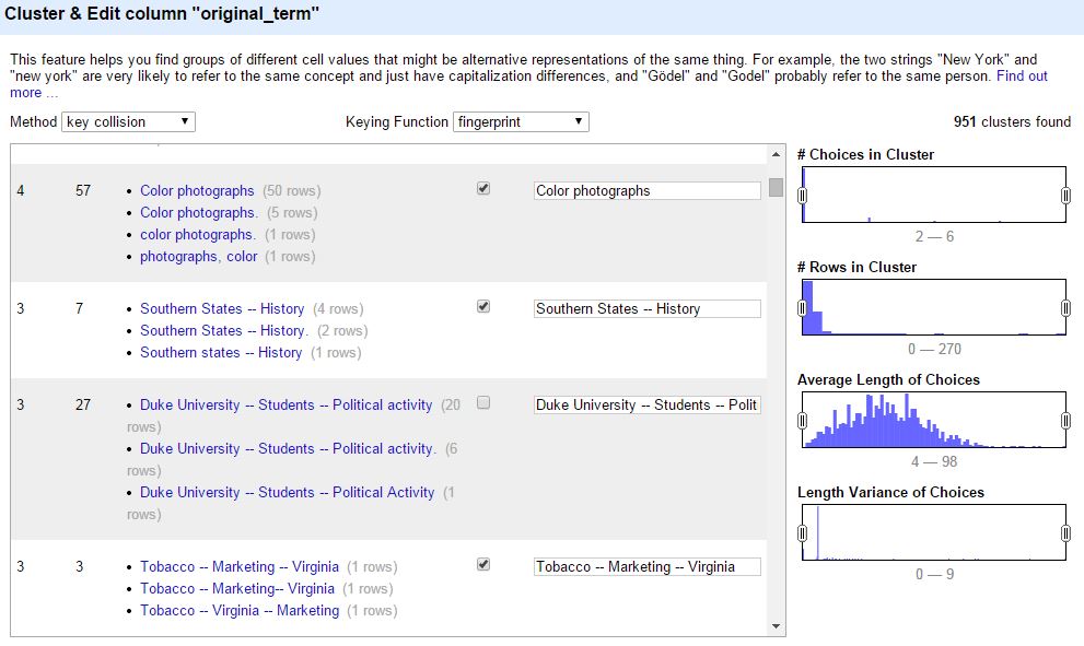
OpenRefine offers several amazing tools for viewing and cleaning data.  For my project, I mostly used the “cluster and edit” feature, which applies several different matching algorithms to identify, cluster, and facilitate clean up of term variants. You can read more about clustering in Open Refine here: Clustering in Depth.

In my list of about 27,000 terms, I identified around 1200 term variants in about 2 hours using the “cluster and edit” feature, reducing the total number of unique values from about 18,000 to 16,800 (about 7%). Finding and replacing all 1200 of these variants manually in EAD or even in Excel would have taken days and lots of coffee.

refine_screeshot
Screenshot of “Cluster & Edit” tool in OpenRefine, showing variants that needed to be merged into a single heading.


In addition to “cluster and edit,” OpenRefine provides a really powerful way to reconcile your data against known vocabularies.  So, for example, you can configure OpenRefine to query the Library of Congress Subject Heading database and attempt to find LCSH values that match or come close to matching the subject terms in your spreadsheet.  I experimented with this feature a bit, but found the matching a bit unreliable for my needs.  I’d love to explore this feature again with a different data set.  To learn more about vocabulary reconciliation in OpenRefine, check out freeyourmetadata.org

 3. Export the cleaned spreadsheet from OpenRefine as an Excel file

Simple enough.

4. Open the Excel file and use Excel’s “XML Map” feature to export the spreadsheet as XML.

I admit that this is quite a hack, but one I’ve used several times to convert Excel spreadsheets to XML that I can then process with XSLT.  To get Excel to export your spreadsheet as XML, you’ll first need to create a new template XML file that follows the schema you want to output.  Excel refers to this as an “XML Map.”  For my project, I used this one: controlaccess_cleaner_xmlmap.xml

From the Developer tab, choose Source, and then add the sample XML file as the XML Map in the right hand window.  You can read more about using XML Maps in Excel here.

After loading your XML Map, drag the XML elements from the tree view in the right hand window to the top of the matching columns in the spreadsheet.  This will instruct Excel to map data in your columns to the proper XML elements when exporting the spreadsheet as XML.

Once you’ve mapped all your columns, select Export from the developer tab to export all of the spreadsheet data as XML.

Your XML file should look something like this: controlaccess_cleaner_dataset.xml

control_access_dataset_chunk
Sample chunk of exported XML, showing mappings from original terms to cleaned terms, type of term, and originating EAD identifier.


5. Use XSLT to batch process your source EAD files and find and replace the original terms with the cleaned terms.

For my project, I bundled the term cleanup as part of a larger XSLT “scrubber” script that fixed several other known issues with our EAD data all at once.  I typically use the Oxygen XML Editor to batch process XML with XSLT, but there are free tools available for this.

Below is a link to the entire XSLT scrubber file, with the templates controlling the <controlaccess> term cleanup on lines 412 to 493.  In order to access the XML file  you saved in step 4 that contains the mappings between old values and cleaned values, you’ll need to call that XML from within your XSLT script (see lines 17-19).

AT-import-fixer.xsl

What this script does, essentially, is process all of your source EAD files at once, finding and replacing all of the old name and subject terms with the ones you normalized and deduped in OpenRefine. To be more specific, for each term in EAD, the XSLT script will find the matching term in the <original_term>field of the XML file you produced in step 4 above.  If it finds a match, it will then replace that original term with the value of the <cleaned_term>.  Below is a sample XSLT template that controls the find and replace of <persname> terms.

XSLT template that find and replaces old values with cleaned ones.


Final Thoughts

Admittedly, cobbling together all these steps was quite an undertaking, but once you have the architecture in place, this workflow can be incredibly useful for normalizing, reconciling, and deduping metadata values in any flavor of XML with just a few tweaks to the files provided.  Give it a try and let me know how it goes, or better yet, tell me a better way…please.

More resources for working with OpenRefine:

“Using Google Refine to Clean Messy Data” (Propublica Blog)

freeyourmetadata.org

On Tour with H. Lee Waters: Visualizing a Logbook with TimeMapper

The H. Lee Waters Film Collection we published earlier this month has generated quite a buzz. In the last few weeks, we’ve seen a tremendous uptick in visits to Duke Digital Collections and received comments, mail, and phone calls from Waters fans, film buffs, and from residents of the small towns he visited and filmed over 70 years ago. It’s clear that Waters’ “Movies of Local People” have wide appeal.

The 92 films in the collection are clearly the highlight, but as an archivist and metadata librarian I’m just as fascinated by the logbooks Waters kept as he toured across the Carolinas, Virginia, and Tennessee screening his films in small town theaters between 1936 and 1942. In the logbooks, Waters typically recorded the theater name and location where he screened each film, what movie-goers were charged, his percentage of the profits, his revenue from advertising, and sometimes the amount and type of footage shown.

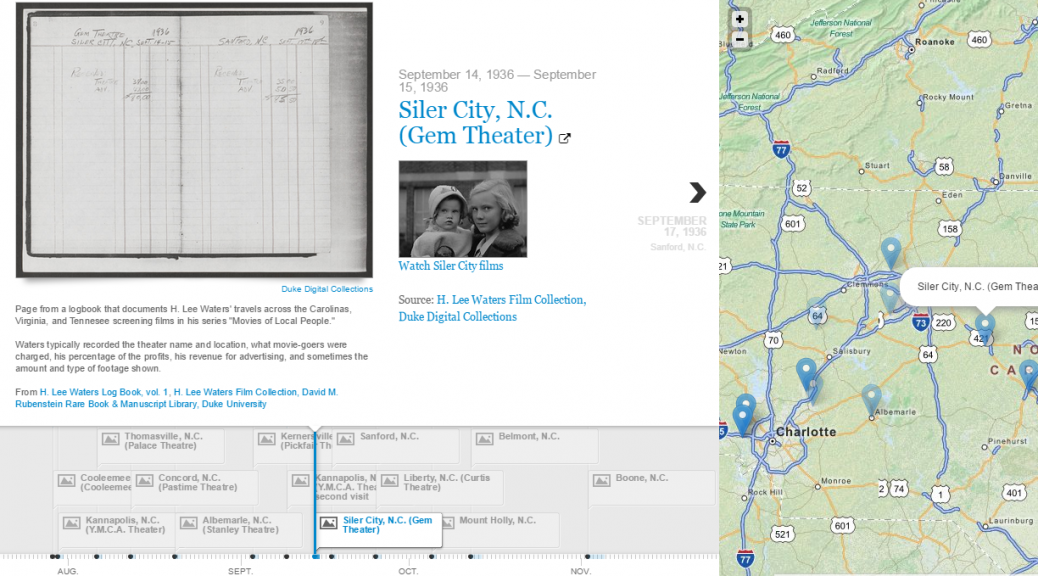
As images in the digital collection, the logbooks aren’t that interesting (at least visually), but the data they contain tell a compelling story. To bring the logbooks to life, I decided to give structure to some of the data (yes, a spreadsheet) and used a new visualization tool I recently discovered called TimeMapper to plot Waters’ itinerary on a synchronized timeline and map–call it a timemap! You can interact with the embedded timemap below, or see a full-screen version here. Currently, the Waters timemap only includes data from the first 15 pages of the logbook (more to come!). Already, though, we can start to visualize Waters’ route and the frequency of film screenings.  We can also interact with the digital collection in new ways:

  • Click on a town in the map view to see when Waters’ visited and then view the logbook entry or any available films for that town.
  • Slide the timeline and click through the entries to trace Waters’ route
  • Toggle forward or backwards through the logbook entries to travel along with Waters

For me, the Waters timemap demonstrates the potential for making use of the data in our collections, not just the digitized images or artifacts. With so many simple and freely available tools like TimeMapper and Google Fusion Tables (see my previous post), it has never been so easy to create interactive visualizations quickly and with limited technical skills.

I’d love to see someone explore the financial data in Waters’ logbooks to see what we might learn about his accounting practices or even about the economic conditions in each town. The logbook data has the potential to support any number of research questions. So start your own spreadsheet and have at it!

[Thanks to the folks at Open Knowledge Labs for developing TimeMapper]

Preview of the W. Duke, Sons & Co. Digital Collection

T206_Piedmont_cards
When I almost found the T206 Honus Wagner

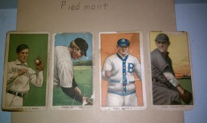
It was September 6, 2011 (thanks Exif metadata!) and I thought I had found one–a T206 Honus Wagner card, the “Holy Grail” of baseball cards.  I was in the bowels of the Rubenstein Library stacks skimming through several boxes of a large collection of trading cards that form part of the W. Duke, Sons & Co. adverting materials collection when I noticed a small envelope labeled “Piedmont.”  For some reason, I remembered that the Honus Wagner card was issued as part of a larger set of cards advertising the Piedmont brand of cigarettes in 1909.  Yeah, I got pretty excited.

I carefully opened the envelope, removed a small stack of cards, and laid them out side by side, but, sadly, there was no Honus Wagner to be found.  A bit deflated, I took a quick snapshot of some of the cards with my phone, put them back in the envelope, and went about my day.  A few days later, I noticed the photo again in my camera roll and, after a bit of research, confirmed that these cards were indeed part of the same T206 set as the famed Honus Wagner card but not nearly as rare.

Fast forward three years and we’re now in the midst of a project to digitize, describe, and publish almost the entirety of the W. Duke, Sons & Co. collection including the handful of T206 series cards I found.  The scanning is complete (thanks DPC!) and we’re now in the process of developing guidelines for describing the digitized cards.  Over the last few days, I’ve learned quite a bit about the history of cigarette cards, the Duke family’s role in producing them, and the various resources available for identifying them.

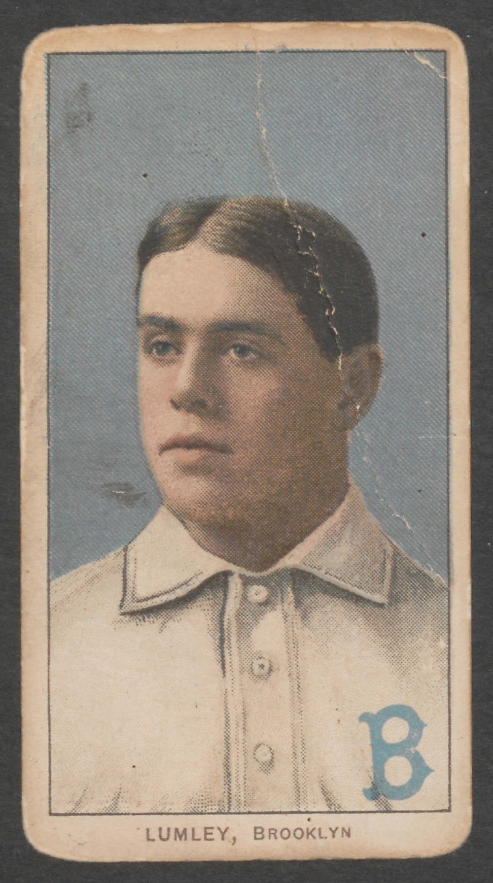
T206 Harry Lumley
1909 Series T206 Harry Lumley card (front), from the W. Duke, Sons & Co. collection in the Rubenstein Library
T206 Harry Lumley card (back)
1909 Series T206 Harry Lumley card (back)


Brief History of Cigarette Cards

A Bad Decision by the Umpire
“A Bad Decision by the Umpire,” from series N86 Scenes of Perilous Occupations, W. Duke, Sons & Co. collection, Rubenstein Library.
  • Beginning in the 1870s, cigarette manufacturers like Allen and Ginter and Goodwin & Co. began the practice of inserting a trade card into cigarette packages as a stiffener. These cards were usually issued in sets of between 25 and 100 to encourage repeat purchases and to promote brand loyalty.
  • In the late 1880s, the W. Duke, Sons, & Co. (founded by Washington Duke in 1881), began inserting cards into Duke brand cigarette packages.  The earliest Duke-issued cards covered a wide array of subject matter with series titled Actors and Actresses, Fishers and Fish, Jokes, Ocean and River Steamers, and even Scenes of Perilous Occupations.
  • In 1890, the W. Duke & Sons Co., headed by James B. Duke (founder of Duke University), merged with several other cigarette manufacturers to form the American Tobacco Company.
  • In 1909, the American Tobacco Company (ATC) first began inserting baseball cards into their cigarettes packages with the introduction of the now famous T206 “White Border” set, which included a Honus Wagner card that, in 2007, sold for a record $2.8 million.
The American Card Catalog
Title page from library’s copy of The American Card Catalog by Jefferson R. Burdick.

Identifying Cigarette Cards

  • The T206 designation assigned to the ATC’s “white border” set was not assigned by the company itself, but by Jefferson R. Burdick in his 1953 publication The American Card Catalog (ACC), the first comprehensive catalog of trade cards ever published.
  • In the ACC, Burdick devised a numbering scheme for tobacco cards based on manufacturer and time period, with the two primary designations being the N-series (19th century tobacco cards) and the T-series (20th century tobacco cards).  Burdick’s numbering scheme is still used by collectors today.
  • Burdick was also a prolific card collector and his personal collection of roughly 300,000 trade cards now resides at the Metropolitan Museum of Art in New York.


Preview of the W. Duke, Sons & Co. Digital Collection [coming soon]

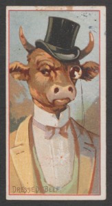
Dressed Beef (Series N81 Jokes)
“Dressed Beef” from Series N81 Jokes, W. Duke, Sons & Co. collection, Rubenstein Library
  •  When published, the W. Duke, Sons & Co. digital collection will feature approximately 2000 individual cigarette cards from the late 19th and early 20th centuries as well as two large scrapbooks that contain several hundred additional cards.
  • The collection will also include images of other tobacco advertising ephemera such as pins, buttons, tobacco tags, and even examples of early cigarette packs.
  • Researchers will be able to search and browse the digitized cards and ephemera by manufacturer, cigarette brand, and the subjects they depict.
  • In the meantime, researchers are welcome to visit the Rubenstein Library in person to view the originals in our reading room.


Analog to Digital to Analog: Impact of digital collections on permission-to-publish requests

We’ve written many posts on this blog that describe (in detail) how we build our digital collections at Duke, how we describe them, and how we make them accessible to researchers.

At a Rubenstein Library staff meeting this morning one of my colleagues–Sarah Carrier–gave an interesting report on how some of our researchers are actually using our digital collections. Sarah’s report focused specifically on permission-to-publish requests, that is, cases where researchers requested permission from the library to publish reproductions of materials in our collection in scholarly monographs, journal articles, exhibits, websites, documentaries, and any number of other creative works. To be clear, Sarah examined all of these requests, not just those involving digital collections. Below is a chart showing the distribution of the types of publication uses.

Types of permission-to-publish requests, FY2013-2014

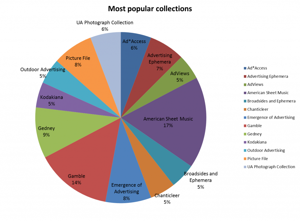
What I found especially interesting about Sarah’s report, though, is that nearly 76% of permission-to-publish requests did involve materials from the Rubenstein that have been digitized and are available in Duke Digital Collections. The chart below shows the Rubenstein collections that generate the highest percentage of requests. Notice that three of these in Duke Digital Collections were responsible for 40% of all permission-to-publish requests:

Collections generating the most permission-to-publish requests, FY2013-2014

So, even though we’ve only digitized a small fraction of the Rubenstein’s holdings (probably less than 1%), it is this 1% that generates the overwhelming majority of permission-to-publish requests.

I find this stat both encouraging and discouraging at the same time. On one hand, it’s great to see that folks are finding our digital collections and using them in their publications or other creative output. On the other hand, it’s frightening to think that the remainder of our amazing but yet-to-be digitized collections are rarely if ever used in publications, exhibits, and websites.

I’m not suggesting that researchers aren’t using un-digitized materials. They certainly are, in record numbers. More patrons are visiting our reading room than ever before. So how do we explain these numbers? Perhaps research and publication are really two separate processes. Imagine you’ve just written a 400 page monograph on the evolution of popular song in America, you probably just want to sit down at your computer, fire up your web browser, and do a Google Image Search for “historic sheet music” to find some cool images to illustrate your book. Maybe I’m wrong, but if I’m not, we’ve got you covered. After it’s published, send us a hard copy. We’ll add it to the collection and maybe we’ll even digitize it someday.

[Data analysis and charts provided by Sarah Carrier – thanks Sarah!]

Mapping the Broadsides Collection, or, how to make an interactive map in 30 minutes or less

Ever find yourself with a pile of data that you want to plot on a map? You’ve got names of places and lots of other data associated with those places, maybe even images? Well, this happened to me recently. Let me explain.

A few years ago we published the Broadsides and Ephemera digital collection, which consists of over 4,100 items representing almost every U.S. state. When we cataloged the items in the collection, we made sure to identify, if possible, the state, county, and city of each broadside. We put quite a bit of effort into this part of the metadata work, but recently I got to thinking…what do we have to show for all of that work? Sure, we have a browseable list of place terms and someone can easily search for something like “Ninety-Six, South Carolina.” But, wouldn’t it be more interesting (and useful) if we could see all of the places represented in the Broadsides collection on one interactive map? Of course it would.

So, I decided to make a map. It was about 4:30pm on a Friday and I don’t work past 5, especially on a Friday. Here’s what I came up with in 30 minutes, a Map of Broadside Places. Below, I’ll explain how I used some free and easy-to-use tools like Excel, Open Refine, and Google Fusion Tables to put this together before quittin’ time.

Step 1: Get some structured data with geographic information
Mapping only works if your data contain some geographic information. You don’t necessarily need coordinates, just a list of place names, addresses, zip codes, etc. It helps if the geographic information is separated from any other data in your source, like in a separate spreadsheet column or database field. The more precise, structured, and consistent your geographic data, the easier it will be to map accurately. To produce the Broadsides Map, I simply exported all of the metadata records from our metadata management system (CONTENTdm) as a tab delimited text file, opened it in Excel, and removed some of the columns that I didn’t want to display on the map.

Step 2: Clean up any messy data..
For the best results, you’ll want to clean your data. After opening my tabbed file in Excel, I noticed that the place name column contained values for country, state, county, and city all strung together in the same cell but separated with semicolons (e.g. United States; North Carolina; Durham County (N.C.); Durham (N.C.)). Because I was only really interested in plotting the cities on the map, I decided to split the place name column into several columns in order to isolate the city values.

To do this, you have a couple of options. You can use Excel’s “text to columns” feature, instructing it to split the column into new columns based on the semicolon delimiter or you can load your tabbed file into Open Refine and use its “split columns into several columns” feature. Both tools work well for this task, but I prefer OpenRefine because it includes several more advanced data cleaning features. If you’ve never used OpenRefine before, I highly recommend it. It’s “cluster and edit” feature will blow your mind (if you’re a metadata librarian).

Step 3: Load the cleaned data into Google Fusion Tables
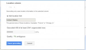
Google Fusion Tables is a great tool for merging two or more data sets and for mapping geographic data. You can access Fusion Tables from your Google Drive (formerly Google Docs) account. Just upload your spreadsheet to Fusion Tables and typically the application will automatically detect if one of your columns contains geographic or location data. If so, it will create a map view in a separate tab, and then begin geocoding the location data.

geocoding_fusion_tables

If Fusion Tables doesn’t automatically detect the geographic data in your source file, you can explicitly change a column’s data type in Fusion Tables to “Location” to trigger the geocoding process. Once the geocoding process begins, Fusion Tables will process every place name in your spreadsheet through the Google Maps API and attempt to plot that place on the map. In essence, it’s as if you were searching for each one of those terms in Google Maps and putting the results of all of those searches on the same map.

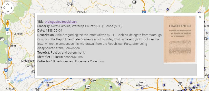
Once the geocoding process is complete, you’re left with a map that features a placemark for every place term the service was able to geocode. If you click on any of the placemarks, you’ll see a pop-up information window that, by default, lists all of the other metadata elements and values associated with that record. You’ll notice that the field labels in the info window match the column headers in your spreadsheet. You’ll probably want to tweak some settings to make this info window a little more user-friendly.

info_window_styled

Step 4: Make some simple tweaks to add images and clickable links to your map
To change the appearance of the information window, select the “change” option under the map tab then choose “change info window.” From here, you can add or remove fields from the info window display, change the data labels, or add some custom HTML code to turn the titles into clickable links or add thumbnail images. If your spreadsheet contains any sort of URL, or identifier that you can use to reliably construct a URL, adding these links and images is quite simple. You can call any value in your spreadsheet by referencing the column name in braces (e.g. {Identifier-DukeID}). Below is the custom HTML code I used to style the info window for my Broadsides map. Notice how the data in the {Identifier-DukeID} column is used to construct the links for the titles and image thumbnails in the info window.

info_window_screen

Step 5: Publish your map
Once you’re satisfied with you map, you can share a link to it or embed the map in your own web page or blog…like this one. Just choose tools->publish to grab the link or copy and paste the HTML code into your web page or blog.

To learn more about creating maps in Google Fusion Tables, see this Tutorial or contact the Duke Library’s Data and GIS Services.